| Work at the Moving Boundary of a Simple Compressible System |
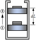
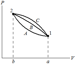
| Work done on the air during a quasi-equilibrium compression process |
| 1W 2 | work from state 1 to state 2 |
| P | pressure |
| V | volume |
| A | area |
| L | length |
| (Eq1) |
|
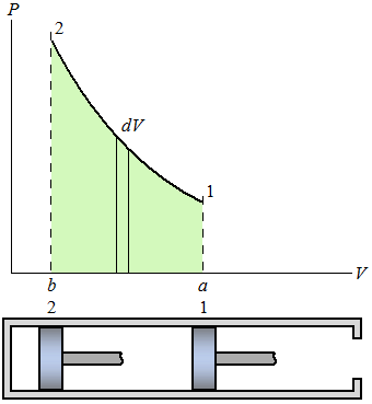
| 1W 2 = | ∫ |
| δW = | ∫ |
| P dV |
| (Eq2) |
|
| ∫ |
| P dV |
| ∫ |
| P dV = V2 − V1 |
| ∫ |
| δW = 1W 2 |